Generative models have been one of the top deep learning trends over the last years. Research efforts have allowed generation capabilities to improve dramatically.

For instance, the SOTA for image synthesis has progressed like this:

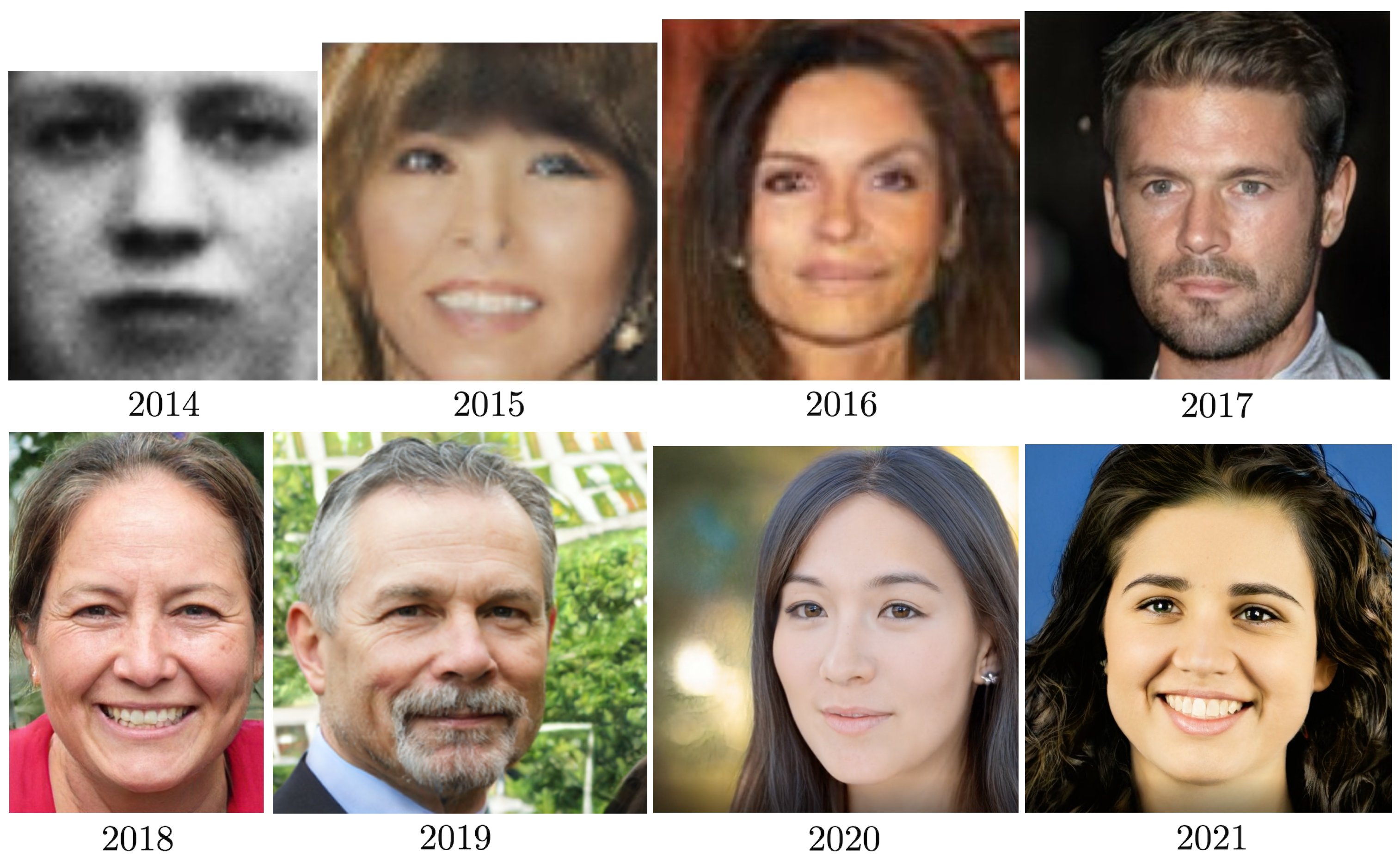
Figure 1: Face generation progress. Image source: Tamay Besiroglu's twitter

Originated in 2014 by Ian Goodfellow, now Director of Machine Learning at Apple, generative adversarial networks (GANs) are the most famous type of generative models. Recently, competitive alternatives like difussion models have arisen, but in this post we are focusing on GANs. The objective is to provide a good understanding of a list of key contributions specific to GAN training.

For the sake of simplicity, we may refer to images as the generation target, but GANs are applicable to many other problems and fields like image to image translation, text to image synthesis, audio synthesis or text to speech, where all the techniques presented are also useful or adaptable. Therefore, every time the term “image” appears in this text it could be substituted by a more generic “data sample” or a term specific to another area.

Introduction

A GAN is composed by two networks: a generator and a discriminator. As its name implies, the generator is the network that creates data, while the discriminator is a classifier specialized in distinguishing real from generated data. The former is the network we are actually interested in whereas the latter is simply a tool that we use while training to help the generator to improve.

In the classic problem that GANs solve, we want to generate data from scratch. We take a set of data samples, belonging to some distribution, as training data. So, let’s say you have a dataset of images of buildings and you wish to generate new images of buildings. Supposing an ideal scenario, where the generator learns to implicitly model the distribution of buildings, you’ll be able to generate different images of the same kind using the generator to indirectly sample from that distribution.

The generator receives a random noise vector sampled from a prior distribution and outputs a new data sample. The discriminator takes an image as input and outputs a scalar as an estimation of the degree of realism of the input.

Each network is trained independently, in alternate steps, with the ratio between the discriminator and generator steps usually ranging from 1 to 5, more often in the low end.

When you train the discriminator, the aim is to make it distinguish between the real and the generated images. The generator is trained to fool the discriminator to make it believe the synthetic images are real; in other words, each weight of the generator should be updated in the direction that makes the critic output a value closer to the real label, usually a 1 after the activation, but it depends on the loss function.

This competition between the generator and the discriminator can be modeled as minimax game that G and D play, with the following value function:

\[\min_G \max_D V(D, G) = \mathbb{E}_{x\sim p_{data}}[\log D(x)] + \mathbb{E}_{z\sim p_z}[\log(1 - D(G(z)))]\]

where:

\(p_{data}\) is the distribution of real images
\(z\) is a random variable distributed as a prior \(p_z\); for example, \(N(0, 1)\)
\(D\) is the discriminator function
\(G\) is the generator function

The solution is a Nash equilibrium where none of the players can take a unilateral action (parameter update) that improves their score.

The discriminator cost is defined as:

\[J^{(D)}(\theta^{(D)}, \theta^{(G)}) = -\frac{1}{2}\mathbb{E}_{x \sim p_{data}} [\log D(x)] -\frac{1}{2}\mathbb{E}_z [\log(1 - D(G(z)))]\]

where:

\(\theta^D\) are the parameters of the discriminator
\(\theta^G\) are the parameters of the generator

It’s the equivalent of a binary cross entropy loss evaluated on a minibatch of real examples, with target 1, and a minibatch of fake examples, with target 0.

The generator cost, when the problem is formulated as a minimax game, is defined as the negative of the cost of the discriminator:

\[J^{(G)} = -J^{(D)} = \frac{1}{2} \mathbb{E_z} \log (1 - D(G(z)))\]

Note that the first term in \(J^{(D)}\), \(E_{x\sim p_{data}} \log D(x)\), can be omited because it doesn’t depend on the parameters of the generator and is irrelevant for the optimizer because its derivative with respect to \(\theta^G\) is always 0.

Training a GAN

In practice, training a GAN can be tricky. There are two main groups of issues one might face:

Instability
Failure to converge

Nowadays, multiple solutions and tweaks have been found to deal with the most common problems.

It might be wise to choose options that add complexity to the discriminator or the loss function over those that add it to the generator, because both have a training cost, but the former are free for production inference.

Most tweaks revolve around the idea of making the discriminator never be too good, such that it can always provide useful gradients to the generator even for images far from the real distribution.

Let’s explore some popular techniques, in chronological order:

Non saturating loss

Also proposed in the original paper [1], it’s an alternative formulation of the generator loss.

Instead of minimizing:

\[J^{(G)} = \frac{1}{2} \mathbb{E_z} \log (1 - D(G(z)))\]

we should minimize:

\[J^{(G)} = -\frac{1}{2} \mathbb{E_z} \log (D(G(z)))\]

Why? The first formulation of the generator cost has a major practical downside. If we plot \(J^{(G)}\) as a function of \(D(G(z))\), we can see that the gradients are close to 0 when the generator is wrong (or unable to fool the critic, at least), which is undesirable when we are training the generator:

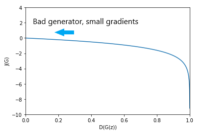
This issue that happens when the generator (or a neural network in general) is unable to learn due to lack of gradients is referred to as the “vanishing gradients problem”.

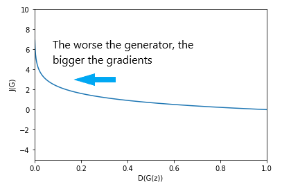
In contrast, with the second formula we have:

Figure 3: non-saturating generator cost plot

But… why do we care about the gradients of \(J{(G)}\) as a function of \(D(G(z; \theta^{G}))\)?

Remember, the chain rule:

If \(h(x) = f(g(x))\), then \(h^{'}(x) = f^{'}(g(x))g^{'}(x)\)

This means that, in this case, the derivative of \(J^{(G)}\) with respect to \(\theta^G\), which we use to know in which direction to update \(G\)’s parameters, is dependant on \(-\log^{'} D(G(z))\) as its first factor, so, for the gradients to flow to the generator during backpropagation, \(-\log^{'} D(G(z))\) shouldn’t be too close to 0. And when do we care more about the gradients of the generator? When it’s wrong. We don’t care that much if the generator doesn’t receive gradients when its purpose of fooling the discriminator is achieved i.e., when \(D(G(z))\) is close to 1. If the output of the generator isn’t that good despite fooling the discriminator, after posterior steps of discriminator training, \(D(G(z))\) will be lower and the generator will receive gradients again.

This is possible because the discriminator loss, with respect to \(D(G(z))\) has this desirable (or not quite undesirable, at least) form:

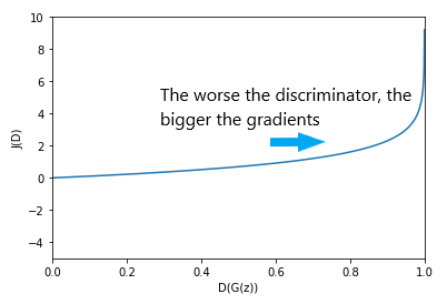
Hence, it doesn’t saturate in the region where it needs to learn more, when \(D(G(z))\) is close to 1.

One-sided label smoothing

One-sided label smoothing [4] is a simplified application of label smoothing [3] to GANs that uses a soft target only for the real label of the discriminator.

In this case, for a binary classifier with targets 0 and 1, what we do is to modify the target for the real examples to be \(1 - \alpha\), a bit lower than 1. A typical value of \(\alpha\) would be 0.1.

As an intuition, we are telling the critic that a real image is “not so real” to prevent overconfidence that could harm the learning process. When the target is 1 nothing prevents the discriminator to predict extremely large logits for real examples (although it has diminishing returns); with one-sided label smoothing if the logits for some samples are extremely high, the discriminator is encouraged to reduce the logits to a lower value that’s closer to \(1 - \alpha\) after the activation.

As noted by Goodfellow et al. [2], it is important to not smooth the labels for the fake samples because it could cause that fake samples in dense regions of the generator implicit distribution have no incentive to move towards the real distribution.

Wasserstein GANs and the importance of discriminator’s gradients

Paper
The WGAN theory in this section is heavily inspired by this awesome post. If you are interested in digging deeper, you won’t regret reading it. I also recommend this one (and every post there!).

In the “non saturating loss” section, we talked about the shape of the loss function with respect to \(D(G(z))\), taking into account the outer log and its arguments. However, it was an oversimplification. The binary cross entropy loss requires the output of \(D\) to be between 0 and 1. This is usually enforced using a sigmoid activation. Indeed, in deep learning libraries like PyTorch, you can find a version of the BCE loss that includes a sigmoid. The sigmoid function has the following form:

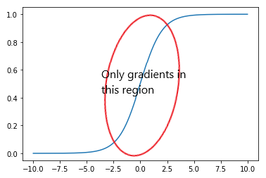
The issue here is that the gradients are concentrated around 0 and the rest of the domain has low gradients. A clever reader may counter that we should fuse the log and the sigmoid and check the combined effect because the derivative can be calculated in one go. Ok, let’s do that.

Let \(S(x) = \frac{e^x}{e^x+1}\) be the sigmoid function and let \(D_2\) be a discriminator that doesn’t include the sigmoid function.

We have \(J^{(G)} = -\mathbb{E_z} \log (S(D_2(G(z))))\)

Applying basic derivative rules we get \(S'(x) = S(x) - S^2(x)\)

Now, we compute the derivate of a fused log + sigmoid:

\[(-log(S(x)))' = -(\frac{1}{S(x)} · S'(x) ) = -(\frac{1}{S(x)} · (S(x) - S^2(x)) ) = -(1 - S(x)) = S(x) - 1\]

Just a sigmoid translated vertically! We can plot this to see \(J'^{(G)}\) as a function of \(D_2(G(z))\):

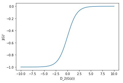
Be aware that the plot above is a derivative. Thus, the gradient vanishes in the right part, for big discriminator logits, when the generator is tricking the discriminator. This is confirmed when we plot the function before the derivative:

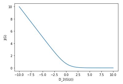
All in all, the graph looks even better once we take into account the sigmoid. Still, we don’t have any certainty about the gradients inside \(D_2\). It turns out that if the supports (regions of the domain where p > 0) of \(p_{data}\) and \(p_g\) (distribution of synthetic data) are disjoint, there exists an perfect discriminator that has no gradients with respect to the input. It hints that we may not want a perfect discriminator, but one kind of good with stable gradients; nevertheless, we’d prefer not having to worry about maintaining a balance by not training \(D\) to optimality.

What can we do to solve this problem and, in general, guarantee that the loss function has gradients everywhere? This is exactly the purpose of the Wasserstein loss.

The Wasserstein Distance is a distance function between probability distributions that has better convergence properties than other distances like the KL divergence or the Jensen-Shannon divergence. It’s also called Earth Mover distance, because it can be seen as the minimal effort required to transform a distribution into another, interpreting each distribution as a pile of earth that needs to be moved until matching the other; the cost is proportional to the amount of earth moved and the distance of movement.

The Wasserstein distance is defined as:

\[W(P_r, P_\theta) = \inf_{\gamma \in \Pi(P_r, P_\theta)} E_{(x, y)\sim \gamma}[||x - y||]\]

where:

\(P_r\) is the distribution of real data.
\(P_\theta\) is the distribution that tries to approximate \(P_r\), in our case the distribution implicitly learned by the generator.
\(\Pi(P_r, P_\theta)\) is the set of all joint distributions \(\gamma\) whose marginal distributions are \(P_r\) and \(P_\theta\). This ensures that every \(\gamma\) is a transport plan to transform \(P_r\) into \(P_\theta\) or viceversa; with \(\gamma(x, y)\) being the amount of mass that needs to be moved from \(x\) (\(P_r\)) to \(y\) (\(P_\theta\)) according to the plan \(\gamma\).

Thanks to the Kantorovich-Rubinstein duality, we can get an equivalent definition easier to deal with:

\[W(P_r, P_\theta) = sup_{||f||_L \le 1} \mathbb{E}_{x\sim P_r}[f(x)] - \mathbb{E}_{x\sim P_\theta}[f(x)]\]

where \(\|f\|_L \le 1\) is the set of all 1-Lipschitz functions. More on this later.

In a nutshell, applied to our case, you can think of the expression above as the maximum difference between \(P_r\) and \(P_\theta\) that can be obtained when using a sufficiently smooth discriminator \(f\).

The Wasserstein Loss is an approximation of the Wasserstein Distance. It is defined as:

Critic: \(\mathbb{E}_{x\sim P_r}(c(x)) - \mathbb{E}_{z\sim P_z}(c(g(z)))\)
Generator: \(\mathbb{E}_{z\sim P_z}(c(g(z)))\)

where \(c\) is the discriminator, now called critic.

The Wasserstein loss eliminates the sigmoid and the logs from the original GAN objective, resulting in a loss function that, intuitively, doesn’t have any obvious limitations to have significant gradients everywhere and should be able to provide feedback to the generator independently of the balance between the generator and the discriminator.

An additional advantage is that the discriminator loss has a correlation with perceptual quality, i.e., a lower loss indicates better image quality.

Strictly speaking, the term “critic” is prefered in this case over “discriminator”, because its output values are unbounded, so you wouldn’t think of the critic as a network that discriminates the inputs as reals or fakes. Anyway, you’ll probably find both terms being used interchangeably.

However, as you may have guessed comparing the Wasserstein loss and metric definitions, for the Wasserstein Loss to be a valid approximation of the Wasserstein Distance the critic needs to satisfy a certain constraint: the output of the critic shouldn’t change much facing small changes of the input, i.e., there must be an upper bound to the gradients of the critic w.r.t. its inputs. This is what is called Lipschitz continuity.

Given two distance functions \(d_X\) and \(d_Y\) with domains \(X \times X\) and \(Y \times Y\), respectively, a function \(f: X \to Y\) is K-Lipschitz continuous if for all \(x_1, x_2 \in X\):
\[d_Y(f(x1), f(x2)) \le Kd_X(x_1, x_2)\]
It’s just constraining the slope of \(f\) to be K at most, by telling that the distance between the function output at two points shouldn’t be more than K times greater than the distance between those two values.

Ideally, the critic should be able to represent every 1-Lipschitz function for our approximation to be guaranteed to be exactly the Wasserstein distance when the critic is trained until convergence. In practice, what we can enforce is that the critic is K-Lipschitz for some unknown K, but, again, it’s not enough.

Imagine that we were able to calculate \(K ⋅ W(P_r,P_\theta)\) for some K. Then, during backpropagation we’d obtain the gradients of \(W(P_r,P_\theta)\) scaled by a constant K, that would turn negligible from an optimization perspective, and we’d be good to go. But… can we calculate \(K ⋅ W(P_r,P_\theta)\)? Not quite, but we can get a decent approximation.

Suppose we have a parametrized family of functions \(\{f_w\}_{w\in W}\), where \(w\) are the weights and \(W\) is the set of all possible weights, that are all K-Lipschitz for some K. Then:

\[\begin{align} \max_{w\in W} E{x\sim P_r}[f_w(x)] − E{x\sim P_\theta}[f_w(x)] &≤ sup_{∥f∥_L\le K} E{x\sim P_r}[f(x)] − E{x\sim P_\theta}[f(x)] \\ &= K ⋅ W(P_r,P_\theta) \end{align}\]

You can think of \(f_w\) as a set of possible functions that our chosen critic architecture can represent. Therefore, we know the distance we can calculate (left side) has an upper bound \(K ⋅ W(P_r,P_\theta)\).

When the supremum is in \(f_w\), the \(\le\) in the equation above becomes an \(=\), meaning that we are not approximating but getting exactly \(K ⋅ W(P_r,P_\theta)\), although we don’t know K.
When it’s not, the smaller \(\{f: ||f||_L \le K \} - \{f_w\}_{w\in W}\) is, the better the approximation; in other words, the accuracy depends on the amount of K-Lipschitz functions not contained in \(\{f_w\}_{w\in W}\).

We still need to know how to force the critic to be K-Lipschitz. In the WGAN paper, the authors suggest to clip the weights of the critic to a fixed box \([-c, c]\) after every optimizer step, which isn’t a particularly good solution in their own words, as it restricts the set of functions that the critic can represent beyond what is intended, making \(\{f_w\}_{w\in W}\) smaller.

The training algorithm recommended by the authors is:

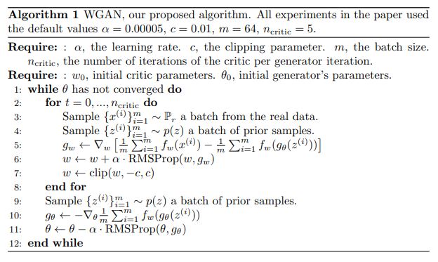
Figure 8: WGAN algorithm. Image source: [5]

Despite its advantages, nowadays the WGAN loss is not a must, and different alternatives like LSGAN or BCE combined with R1 GP are widely used with success.

WGAN-GP

Paper

The weight clipping strategy previously mentioned comes with a set of problems:

If the clipping window is too small, the Wasserstein Distance approximation is poor because the critic is too constrained and the gradients can vanish.
If it’s too wide, training is unstable.

The authors go further and expose a variety of issues that happen training to optimality on toy datasets:

The critic learns simple functions that fail to capture complex properties of the data distribution.
High sensibility to the choice of the clipping window \([-c, c]\), requiring detailed tuning to avoid exploding (high \(c\)) and vanishing (low \(c\)) gradients.
Using softer constraints like L1 or L2 weight decay doesn’t help.
Adding batch normalization layers to the critic is useful but, even then, at least very deep critics often fail to converge.

Here we can see how decreasing \(c\) an order of magnitude (from 0.1 to 0.01) is enough to pass from exploding to vanishing gradients:

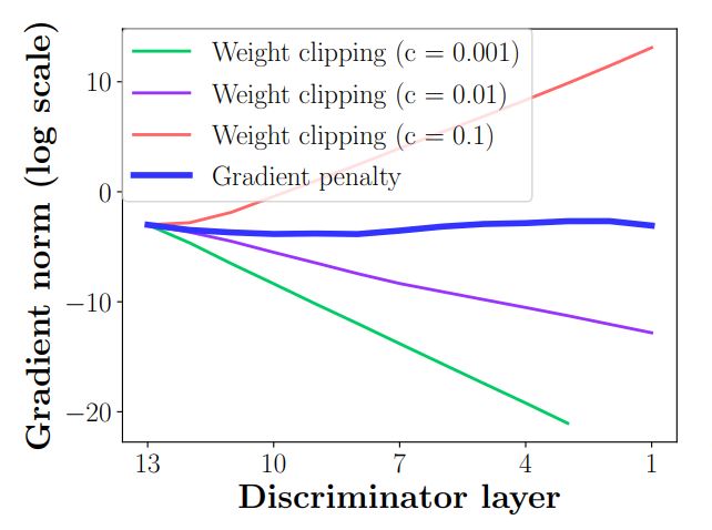
Figure 9: WGAN sensibility to the choice of the clipping window. Image source: [5]

As expected, the problem is less severe at the start of backpropagation (higher discriminator layer indexes) than at the end. The gradient penalty line corresponds to the solution presented in the paper, which we’ll discuss soon. It has to be noted that the comparison is made using critics without batch normalization, not the best scenario for a weight clipped critic.

A gradient penalty is a term added to the critic loss function that encourages the norm of the gradients of the critic w.r.t. its inputs to be as close to 1 as possible. The critic objective becomes:

\[\mathbb{E}_{\tilde{x}\sim P_g}[D(\tilde{x})] - \mathbb{E_{x\sim P_r}}[D(x)] + \lambda \mathbb{E}_{\hat{x}\sim P_{\hat{x}}}[(||\nabla_{\hat{x}}D(\hat{x})||_2 - 1)^2]\]

A solid value for the gradient penalty coefficient is \(\lambda = 10\), but the reader is advised to test a few values above and below if it doesn’t work well for their use case.

The use of batch normalization in the critic is discouraged, given that the GP works on a sample level and doesn’t take into account the correlations between examples introduced by BN. Layer normalization is a sound alternative because it doesn’t normalize across the batch dimension.

We still need to define \(P_{\hat{x}}\), the distribution used to sample the inputs of the critic to calculate the gradient penalty. Every sample of \(P_{\hat{x}}\) is a linear interpolation between a real and a fake sample:

\[\hat{x} = \epsilon x + (1 - \epsilon)\tilde{x}, \text{with } x\sim P_r, \tilde{x}\sim P_g, \epsilon\sim U[0, 1]\]

What’s the reason of this choice?

Enforcing the unit gradient norm constraint everywhere is intractable. To open the door to an alternative, the following is proven (see Apendix of the paper):

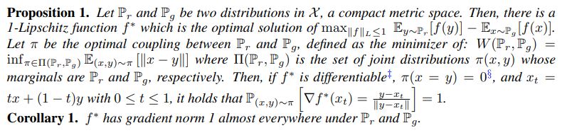
Figure 10: WGAN-GP proposition about norm of the gradients. Image source: [6]

Remember from the Wasserstein GAN section, \(\pi\) is the optimal transport plan that defines how to transform \(P_r\) into \(P_g\) and \(f^*\) is the optimal critic that is used to compute the actual Wasserstein Distance. Then, \(x_t\) is a linear interpolation between points of \(P_r\) and \(P_g\) coupled by the optimal transport plan. Therefore, what is proven is that in the function that the optimal critic represents, there are straigth lines with gradient norm 1 between \(P_r\) and \(P_g\) that connect the points coupled by the optimal transport plan.

The gradient penalty incentivizes the critic to have gradient norm 1 along every straight line between \(P_r\) and \(P_g\).

In conclusion, the gradient penalty encourages the critic to satisfy a condition that the optimal (with regards to the Wasserstein Distance) critic meets. Of course, it isn’t the same as incentivizing the critic to be exactly that “optimal” critic \(f^*\).

The full training algorithm included in the paper is:

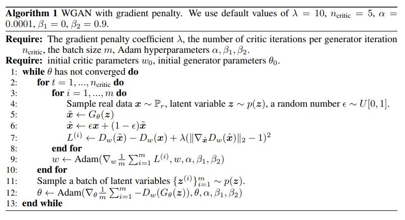
Figure 11: WGAN-GP algorithm. Image source: [6]

The experiments show that a WGAN critic trained with gradient penalty doesn’t suffer any of the issues enumerated for weight clipping and outperforms it. It would have been interesting to see a comparison with a weight clipped critic that incorporates BN layers.

Two Time-scale Update Rule (TTUR)

Paper

This paper studies convergence while dealing with stochastic gradients, corresponding to a realistic mini-batch learning scenario, unlike previous work.

In practice, training with a two time-scale update rule implies choosing separate learning rates for the generator and the discriminator, tipically lower for the generator.

The authors prove that GANs trained with TTUR converge to a Nash equilibrium for both stochastic gradient descent and Adam.

An additional (and huge) contribution was the introduction of a new metric, the Frechet Inception Distance (FID), that became the de facto standard for measuring GAN performance. However, it’s beyond the scope of this article.

Spectral normalization

Paper

One of the top contributions towards stabilizing the traning of the discriminator. Spectral normalization controls the Lipschitz constant of the discriminator function by constraining the spectral norm of each layer.

For a WGAN, we saw that Lipschitz continuity is a requirement to ensure a good approximation of the Wasserstein Distance that has desirable convergence properties. In this case, the authors don’t use the Wasserstein Loss, but the original GAN loss with the non saturating generator loss. Still, they defend the need to constrain the gradients of the discriminator and force it to be K-Lipschitz because the derivative of the optimal discriminator is unbounded.

Moreover, it seems reasonable to think that restricting the maximum gradient of the discriminator should result in more balanced gradients provided to the generator and make it harder to reach a plateau during training.

The difference between spectral normalization and previous methods that control the Lipschitz constant of the discriminator, is that SN is able to control it outside the neighboorhoods of the training and synthetic examples.

Now, we are going to see how to perform spectral normalization, but first let’s review some math concepts in order to make the explanation easily understandable for engineers like me.

A norm is a function from a vector space to the set of non-negative real numbers, i.e. its input is a vector and its output is a number greater than or equal to zero, that corresponds to the intuition of the length of a vector. Well, if you are here you probably knew it already. But… what about a matrix norm?

We could define a matrix norm similarly to a vector norm, that operates element-wise over the flattened matrix. However, we are more interested in a different kind called “matrix norms induced by vector norms” that can be defined using vector norms.

Let \(K\) be a field of real or complex numbers, \(A\) be a mxn matrix (\(A \in K^{m\times n}\)) and \(x\) be any non-zero vector in \(K^n\), the matrix norm induced by the p-norm (\(1 \leq p \leq \infty\)) is defined as:

\[|| A ||_p = sup_{x != 0} \frac{||Ax||_p}{||x||_p}\]

It measures how much the linear transformation defined by A can stretch a vector. Imagine that \(A\) is a weight matrix of a linear layer \(g\) of a DNN. The result of the induced matrix p-norm would be the quotient between the norm of the output and the norm of the input, for the input that maximizes it; thus, it would give us an idea of how much \(g\) can potentially increase the magnitude of the inputs.

The matrix norm induced by the L2 norm is also called spectral norm, corresponds to the largest singular value of \(A\) and is denoted \(\sigma(A)\):

\[|| A ||_2 = \sigma(A) = sup_{x != 0} \frac{||Ax||_2}{||x||_2} = sup_{||x||_2 = 1} ||Ax||_2\]

Given a function \(g\), the Lipschitz norm \(\|g\|_{Lip}\) is equal to \(sup_h\sigma(\nabla g(h))\)

For a linear layer \(g(h) = Wh, \|g\|_{Lip} = sup_h\sigma(\nabla g(h)) = sup_h\sigma(W) = \sigma(W)\)

Suppose we have a discriminator that is a composition of linear layers (without bias, for simplicity) and activations:

\[f(x; \theta) = g_{L+1}(a_L(g_L(a_{L-1}(g_{L-1}(...a_1(g_1(x))...))))) = W^{L+1}a_L(W^L(a_{L-1}(W^{L-1}(...a_1(W^1x)...))))\]

where:

\(\{g_1, ..., g_L, g_{L+1}\}\) are the linear layers.
\(\theta = \{W^1, ..., W^L, W^{L+1}\}\) are the learnable parameters, \(W^l \in R^{d_l\times d_{l-1}}, W^{L+1} \in R^{1\times d_L}\)
\(a_l\) is element-wise non-linear activation function.

Then:

Assuming that the activation functions \(a_l\) are 1-Lipschitz. It’s easy to see that some popular activation functions like ReLU or LeakyReLU are Lipschitz, more specifically these examples are 1-Lipschitz as they have a max gradient 1 constant after x=0.
Using the property that \(|| g_1 \circ g_2 ||_{Lip} \leq || g_1 ||_{Lip} · || g_2 ||_{Lip}\). The composition of two functions at most can stretch an input the product of the max stretch that every function can apply to an input; it’d be an equality when the input that is most stretched by \(g_1\) is the same as the input that is most stretched by \(g_2\).

…the Lipschitz norm of the discriminator has an upper bound given by the product of the Lipschitz norms of the layers and activations:

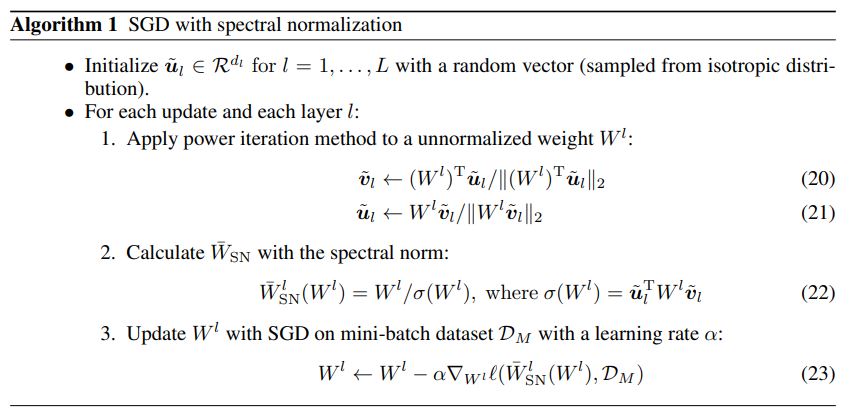
\[||f||_{Lip} \leq ||g_{L+1}||_{Lip} · ||a_L||_{Lip} · ||g_{L-1}||_{Lip} · ... · ||a_1||_{Lip} · ||g_1||_{Lip} = \prod_{l=1}^{L+1} ||g_l||_{Lip} = \prod_{l=1}^{L+1} \sigma(W^l)\]

To perform spectral normalization, we just need to divide each weight matrix W by its spectral norm:

\[\hat{W_{SN}}(W) = \frac{W}{\sigma(W)}\]

After the normalization, the layers with the updated weight matrices have all spectral norm 1, (\(\sigma(W_{SN}(W)) = 1\)). Therefore, the Lipschitz norm of the normalized discriminator has an upper bound equal to 1:

\[||f||_{Lip} \leq = \prod_{l=1}^{L+1} \sigma(W_{SN}(W_l)) = 1\]

You might wonder what happens with convolutional layers. The weight matrix of a convolutional layer can be transformed into an equivalent matrix (but dependant on the input size) of a fully connected layer. However, the authors do something different that turns out to work better: they treat the convolutional weight \(W \in R^{d_{out}×d_{in}×h×w}\) as a 2d matrix of dimension \(d_{out}\times(d_{in}hw)\) and calculate the SN of that matrix.

There’s just one issue to solve. Computing a singular value decomposition for each weight matrix at each step is quite costly. Instead, the recommended approach is to use the power iteration method to estimate the largest singular value. One round of the power iteration algorithm is shown to be enough in practice and cheaper than the WGAN-GP computation. For more information, refer to appendix A of the paper, [9] or the PyTorch implementation.

Figure 12: SN algorithm. Image source: [8]

Experiments show the superiority of SN over weight normalization, weight clipping and gradient penalty, in absence of complimentary techniques like batch normalization or weight decay:

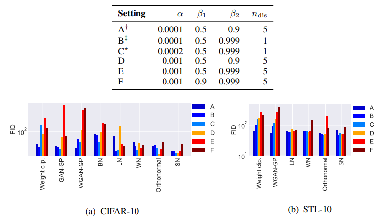
Figure 13: Comparison of FIDs (lower is better) on CIFAR-10 and STL-10 with different methods and hyperparameters. Image source: [8]

Furthermore, SN looks more robust to the hyperparameter choice (\(\alpha\): learning rate, \(\beta_1\): Adam exponential decay rate for the first moment estimates, \(\beta_2\): Adam exponential decay rate for the second moment estimates, \(n_{dis}\): number of discriminator updates per generator update). One could argue that the comparison against weight clipping without BN is rigorous but not fair or too convenient; anyway, it’s common knowledge that gradient penalty tends to work better than weigth clipping + BN, so the edge of SN over GP should be enough to provide an idea of the power of the first one.

An additional advantage is that SN is independent of the rank of each weight matrix, because the Lipschitz constant that is enforced only depends on the largest singular value and the rank is equal to the number of singular values.

Spectral normalization is still widely used today in many GAN architectures. Later work has successfully applied it to the generator too but its convenience is more controversial. Nevertheless, it’s not present in any version of StyleGAN, the state of the art GAN for unsupervised image synthesis, where its effect is slightly negative over the discriminator and null over the generator.

Convergence and R1 GP

Paper

Previous work had proven local convergence of GAN training for absolutely continuous data and generator distributions. However, it wasn’t known if absolute continuity is a necessary condition. This paper proved that it is.

Nevertheless, assuming absolute continuity isn’t realistic. It is accepted that the distributions of data like images lie on low dimensional manifolds. This means, intuitively (sorry, mathematicians), that they don’t need all the representational power given by the number of dimensions actually used to represent the data. It also makes more likely one situation we wanted to avoid: the supports of the real and generated distributions could be disjoint, opening the door to the discriminator to be perfect and kill generator learning.

All of the above led the authors to study convergence under a more realistic scenario of distributions not absolutely continuous, that require regularization techniques. They arrived to the following conclusions:

WGAN an WGAN-GP don’t guarantee convergence when the number of discriminator updates per generator update is finite, even for absolutely continuous distributions.
Gradient penalty on real data only (R1 GP) ensures local convergence.
Gradient penalty on fake data only (R2 GP) ensures local convergence.
Other techniques like instance noise, zero-centered gradient penalties and consensus optimization also lead to convergence.

R1 GP

Suppose we are training a minimalist GAN called Dirac-GAN, composed by a generator distribution \(p_\theta = \delta_\theta\) and a linear discriminator \(D_{\psi}(x) = \psi · x\), with the data distribution \(p_D\) concentrated at 0. Further suppose we are near the equilibrium point of the GAN game.

At a certain iteration of generator training, the discriminator signals the generator the direction to move towards the real distribution:

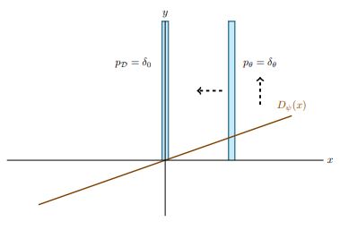
Figure 14: Dirac-GAN, generator distribution approaching real distribution. Image source: [10]

Then, the parameters of the generator are updated. At this moment, the generated distribution is very close to the real distribution. Next, we perform a discriminator step. It must learn to tell two very similar distributions apart. As a consequence, a small variation in the input should produce very different outputs; in other words, the slope or the gradient of \(D(x)\) w.r.t. \(x\) must be big:

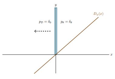
Figure 15: Dirac-GAN, generator distribution similar to real distribution. Image source: [10]

When we train the generator again, that big slope is backpropagated to the generator, that moves away from the real distribution.

Recall from the non saturating loss section, using standard parameters notation, the gradients of D(G(z)) w.r.t. the parameters of the generator depend on the gradients of D w.r.t. its input (first term in the equation below):
\[\frac{\partial D(G(z))}{\partial \theta^G} = \frac{\partial D(G(z))}{\partial G(z)} · \frac{\partial G(z)}{\partial \theta^G}\]

Well, it looks like something is not working as desired. Where’s the problem?

We expect the equilibrium discriminator to have zero slope on the true distribution, so that a generator whose implicit distribution is very close or even equal isn’t pushed away. The reality is that nothing in our framework encourages the discriminator to follow the aforementioned behaviour. It seems we need to incentivize the discriminator somehow to have small gradients when evaluated on real data. This is exactly the role of the \(R_1\) gradient penalty:

\[R_1(\psi) = \frac{\gamma}{2}\mathbb{E}_{x\sim p_{data}}[||\nabla D_{\psi}(x)||^2]\]

where \(\gamma\) is an hyperparameter that assigns a weight to the GP inside the loss function of the discriminator. As explained, it penalizes the deviation from zero of the gradients of the discriminator when evaluated on real data.

You could still hold some doubts:

Isn’t a linear discriminator too limited?
No, the researchers showed that the class of linear discriminators is as powerful as the class of all real-valued functions for our example.
Isn’t the R1 GP detrimental to discriminator training? How would a bad discriminator learn if it’s incentivized to have small gradients when evaluating real data?
This shouldn’t be a problem! Be aware we are talking about the gradients of the discriminator w.r.t. the inputs. We only care about the gradients of the discriminator with respect to its input when we train the generator; to update the discriminator we are only interested in the gradients of the discriminator w.r.t. its parameters.

An equivalent gradient penalty \(R_2\) over the discriminator gradients on the generator distribution is shown to share the same local convergence properties:

\[R_2(\psi) = \frac{\gamma}{2}\mathbb{E}_{x\sim p_{\theta}}[||\nabla D_{\psi}(x)||^2]\]

The R1 GP is currently, as of May 2022, the go-to regularizer for GAN training.

Adaptive discriminator augmentation (ADA)

Paper

Training a GAN using a small dataset entails a harder task. The discriminator is prone to overfit to the training examples, becoming overconfident before the generator has learned as much as it could.

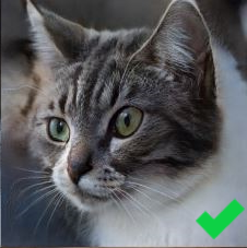
Dataset augmentation is the default remedy to prevent overfitting and alleviate/delay the issue at the very least. For a GAN we must be especially careful with the augmentations that we choose since we expect that their effect is reflected in the generated images. We tipically perform data augmentation adhering to the following rules:

Use only augmentations that make sense for the dataset we are dealing with, i.e. transformations that result in an image that still belongs to the target distribution. For instance, we would flip a face horizontally but not vertically.
Only augment the real images

Source	Original image	Transformation	Transformation
Dataset (real)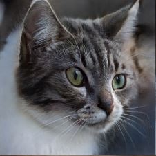
Generator (fake)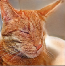

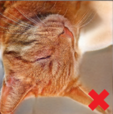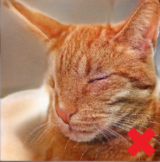
Figure 16: example of valid augmentations according to traditional scheme

What if I tell you that we don’t need to be that strict and, indeed, we can leverage a diverse set of augmentations to delay discriminator overfitting, while preventing them from leaking to the generated images?

First, we need to know how to apply augmentations that don’t leak. The authors find that, surprisingly, it’s possible if we augment any image that the discriminator evaluates, not only the real images but also the synthetic ones.

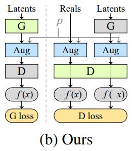
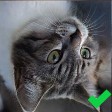
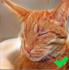
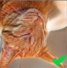
Figure 17: ADA Architecture. Image source: [11]

Source	Original image	Transformation	Transformation
Dataset (real)
Generator (fake)

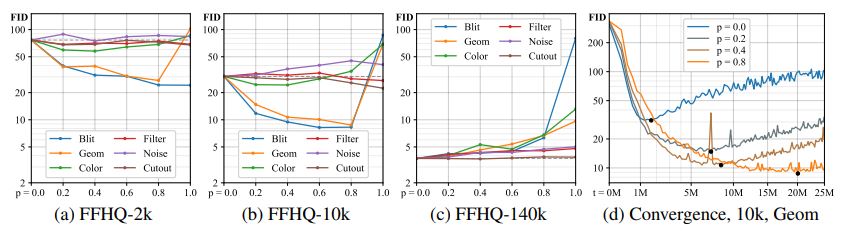
Figure 18: valid augmentations with ADA

For certain transformations, a constraint over the augmentation strength, the probability \(p\) that a given transformation is applied to any single image, is needed too. It depends on the nature of the specific transformation; some are such that allow the discriminator to draw conclusions about the similarity of the original distributions only looking at the augmented distributions. For example, isotropic scaling with log-normal distribution doesn’t leak even for \(p = 1\) whereas more problematic augmentations like random rotations need \(p\) to stay below 0.8 to ensure no leaking.

The last restriction is that the augmentations must be differentiable, since they are applied to the generated images (in the middle of a step).

An interesting property is that if we apply a sequence of augmentations that don’t leak individually, the full pipeline doesn’t leak either. Thanks to it, we’ve got a powerful tool to combat overfitting: we just need to find the maximum “non-leaking” strength \(p\) for each augmentation and then build a diverse pipeline.

Selection of augmentations

The paper studied five groups of transformations:

Pixel blitting: horizontal flips, 90º rotations and integer translation.
More general geometric transformations, like isotropic scaling or arbitrary rotations.
Color transforms: alteration of hue, brightness, …
Image-space filtering: modify the content depending on its frequency.
Image-space corruptions: additive noise and cutout.

The transformations in the pixel blitting group were analyzed separately because they are more “clean” than the rest of the geometric transformations, as they only move pixels without requiring any combination with neighboors.

Because groups 1 and 2 are both geometric transformations, any of these operations can be expressed as a matrix multiplication between a special 3x3 matrix that defines an affine transformation and a size 3 column vector, containing the pixel coordinates and a 1. The first two columns of the 3x3 matrix correspond to a linear transformation, while the third is a translation vector. For example, the transformation matrix for the translation operation is:

\[\begin{bmatrix} 1 & 0 & tx\\ 0 & 1 & ty\\ 0 & 0 & 1 \end{bmatrix}\]

where tx and ty are the magnitude of the translation along the axis x and y.

If we need to apply a set of geometric transformations we can compute beforehand a single transformation matrix by multiplying the sequence of transformation matrices of the operations involved.

The conclusions extracted from the independent analysis of the augmentations were:

The optimal value of \(p\) is highly dependant on the dataset size; the smaller the dataset, the higher the optimal p. This implies that for a sufficiently large dataset, the optimal p is 0, ADA isn’t useful.
Most benefits come from transformation groups 1 and 2, while 3 helps a bit. Therefore, the recommendation is to discard groups 4 and 5.

Figure 19: (a-c) Impact of p for different augmentation categories and dataset sizes. The dashed gray line indicates baseline FID without augmentations. (d) Convergence curves for selected values of p using geometric augmentations with 10k training images. Image source: [11]

The algorithm

We don’t want to apply the augmentation pipeline with a high probability since the start of training, it would make learning too slow at the very least. Instead, we should begin with p=0 and modify this value attending to the degree of overfitting of the discriminator: increase p a fixed amount when D is overfitting too much and otherwise decrease it by the same amount.

The researchers decided to use a common value of p but randomize independently. For example, when p=0.4 the transformation “vertical flip” will be applied 40% of the iterations and the transformation “integer translation” will be applied 40% of the iterations too, but in a specific iteration it can happen that the first is applied and the second is skipped, or viceversa, due to the independent randomization.

How do we know if the discriminator is overfitting?

If we take a look at the real and the generated distribution during a training run, we can see how the best FID is achieved right before the distributions cease to overlap; after it, the FID gets progressively worse. This is just an example but the behaviour seems to be consistent across datasets, at least with the configurations used in the experiments presented in the paper.

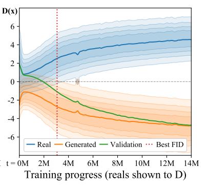
Figure 20: overlap between distributions. Image source: [11]

The rise of FID can be interpreted as a clear sign of discriminator overfitting, but of course we can’t calculate the FID every iteration; we don’t mind, we have a proxy: the overlap between the distributions measured in terms of the discriminator raw outputs. We just need to build an overfitting metric based on the output logits. The authors propose two heuristics:

\[r_v = \frac{\mathbb{E}[D_{train}] - \mathbb{E}[D_{validation}]}{ \mathbb{E}[D_{train}] - \mathbb{E}[D_{generated}]} \\ r_t = \mathbb{E}[sign(D_{train})]\]

In both cases, r = 0 means no overfitting and r = 1 indicates complete overfitting.

Finally, we need a threshold \(r_{target}\) to decide the values of the metric that imply “too much overfitting”. For instance, if our overfitting metric is \(r_t\) and \(r_{target} = 0.6\), we interpret that the discriminator is overfitting too much when more than 60% of the output logits are positive (> 0) for real images.

In summary, we would proceed as follows:

Before training:
- Choose an overfitting metric \(r_x \in \{r_t, r_v\}\).
- Choose \(r_{target}\). The recommended value is 0.6 when the metric is \(r_t\).
- Choose \(p_{inc}\), the increment/decrement added to p at each step. The authors select a value such that it would take no less that 500k images for p to rise from 0 to 1.
Inside the training loop:
- Every 4 iterations, compute \(r_{x}\).
- If \(r_x > r_{target}\), update \(p = p + p_{inc}\).
- Else, update \(p = p - p_{inc}\).

The practitioner should be aware that the heuristics have been tested with specific choices of loss function, architecture, hyperparameters and so on. If you are intending to apply ADA together with a different configuration, it surely has great potential still, but you should assess if the heuristics are appropriate and find an alternative rule in case they aren’t. For instance, the heuristic \(r_t\) could be a bad choice when you are relying on a Wasserstein loss.

Results

ADA delivers an impressive improvement for GANs trained on small to medium-sized datasets, when compared to a then SOTA StyleGAN 2 baseline. The boost is obviously inversely proportional to the dataset size:

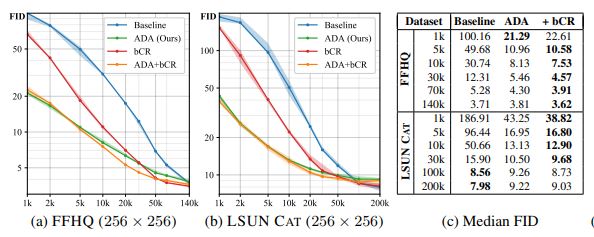
Figure 21: FID as a function of training set size, reported as median/min/max over 3 training runs. Image source: [11]

These results were obtained training from scratch. When using transfer learning, the improvement is moderate but still noticeable.

References

[1] I. Goodfellow, J. Pouget-Abadie, M. Mirza, B. Xu, D. Warde-Farley, S. Ozair, A. Courville, and Y. Bengio. Generative Adversarial Networks. In NIPS, 2014.

[2] I Goodfellow. Nips 2016 tutorial: Generative adversarial networks. CoRR, abs/1701.00160.

[3] Christian Szegedy, Vincent Vanhoucke, Sergey Ioffe, Jon Shlens, and Zbigniew Wojna. Rethinking the inception architecture for computer vision. In Proceedings of the IEEE conference on computer vision and pattern recognition, pages 2818–2826, 2016.

[4] Salimans, T., Goodfellow, I., Zaremba, W., Cheung, V., Radford, A., and Chen, X. (2016). Improved techniques for training gans. In Advances in Neural Information Processing Systems, pages 2226–2234

[5] M. Arjovsky, S. Chintala, and L. Bottou. Wasserstein gan. CoRR, abs/1701.07875, 2017.

[6] I. Gulrajani, F. Ahmed, M. Arjovsky, V. Dumoulin, and A. C. Courville. Improved training of Wasserstein GANs. CoRR, abs/1704.00028, 2017.

[7] Martin Heusel, Hubert Ramsauer, Thomas Unterthiner, Bernhard Nessler, Gunter Klambauer, and Sepp Hochreiter. GANs trained by a two time-scale update rule converge to a nash equilibrium. CoRR, abs/1706.08500, 2017.

[8] T. Miyato, T. Kataoka, M. Koyama, and Y. Yoshida. Spectral normalization for generative adversarial networks. CoRR, abs/1802.05957, 2018.

[9] Gene H Golub and Henk A Van der Vorst. Eigenvalue computation in the 20th century. Journal of Computational and Applied Mathematics, 123(1):35–65, 2000.

[10] L. Mescheder, A. Geiger, and S. Nowozin. Which training methods for GANs do actually converge? CoRR, abs/1801.04406, 2018.

[11] Tero Karras, Miika Aittala, Janne Hellsten, Samuli Laine, Jaakko Lehtinen, Timo Aila. Training Generative Adversarial Networks with Limited Data. CoRR, abs/2006.06676, 2020.

[12] https://twitter.com/tamaybes/status/1450873331054383104

[13] https://www.alexirpan.com/2017/02/22/wasserstein-gan.html

[14] Weng, Lilian. From GAN to WGAN. lilianweng.github.io, 2017.

[15] https://pytorch.org/docs/stable/_modules/torch/nn/utils/parametrizations.html#spectral_norm